My Dream Car

What to do: Create a new Excel worksheet like the one below.

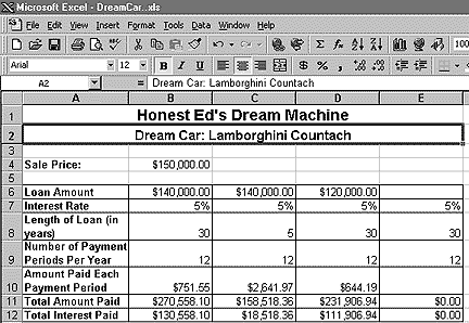This Excel worksheet is designed to calculate interest and total payment for a purchase, based on different loan terms.  This example is in dollars but you may create yours for Yen or any other currency, the formulae will remain the same.

Follow these time-saving tips:

Worksheet Titles: To create a bold face and centered worksheet title, type the title in column A and press Enter. Highlight columns A through E and then click the Merge and Center button on Microsoft Excel's Formatting toolbar. Click the Bold button. Increase the font size of the text to 14.

Word Wrap: Enter cell contents in column A. To turn on word wrap, highlight all cells in which text must wrap (A6:A12) then right-click the highlighted cells. Click the Alignment tab, then select Wrap text in the Text control section.

Column Width: To adjust column width, double click the column boundary to the right of a column heading. To create columns of uniform width, select those columns, choose Column from the Format menu, choose Width, then enter a value, e.g. 14.

Formatting Currency: Format cells B4, B6, B10, B11, and B12 as Currency, by selecting B4, then pressing the Ctrl key while clicking the other cells. Right-click on a highlighted cell, then choose Format Cells from the pop-up menu. Click the Number tab and choose Currency.

Saving Work: Turn on AutoSave to have Microsoft Excel save a workbook automatically at a time interval that you specify. If AutoSave is not available from the Tools menu, choose Add-Ins from the Tools menu, place a check mark in the AutoSave Add-Ins dialog box, click OK. Then choose AutoSave from the Tools menu to specify the time interval for Automatic Save. Now Microsoft Excel will pop up save reminders.

Step B
Adding Formulas

What to do :
Follow these time-saving tips for adding formulas:

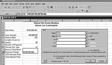This example shows Excel's Periodic Payment Function data input window. Use the steps below to insert a PMT formula into your spreadsheet

PMT Function: In Cell B10 paste Microsoft Excel's PMT function (Periodic Payment Function). Click cell B10, then choose Function from the Insert menu. Select Financial from the Function Category list, then choose PMT from the Function Name list. Click OK.

Type the following cell references in the PMT dialog box. For Rate (the interest rate per period for the loan), type =B7/B9; for Nper (the total number of loan payments), type =B8*B9; for Pv (loan amount), type =B6. Choose OK.

Excel returns a negative number to indicate that you are making a payment.

Note: To work with positive numbers on the worksheet, calculate PMT as follows: =PMT(rate,nper,-pv).

"Total Amount Paid" Formula: In B11, type the following formula, which will calculate the total amount paid for a loan: =SUM(B10*(B8*B9)), where B10=PMT (i.e., the amount paid each payment period) and B8*B9 =nper (the total number of loan payments).

"Interest Paid" Formula: In B12, type the following formula which calculates the total amount of interest paid: =SUM(B11-B6), which is the total amount paid minus the loan amount.

Showing Formulas: To have Excel show formulas, rather than formula results, choose Options from the Tools menu; click the View tab, then select the Formulas check box. To display formula results, clear the check box.

Once you format the cell contents of column B, entering appropriate formulas where necessary, you can copy cell content and format to columns C and D using Autofill or Fill Right.

Step C
Reality Check

What to do: Once your worksheet is set up, you can pose different "what if" questions about your loan to see how the total amount of interest paid might change. For example, what if the interest rate was 4% and the length of the loan was ten years? What would your monthly payment be? How much interest would you pay over the life of the loan? Using one of the duplicate columns, change one of the values, such as the interest rate.  Note the differences that makes.  Now do it again but this time change the number of years and so.

Step D

Open a Word document and type a report on this spreadsheet activity.  Specifically write about the following questions:

• What effect does changing the length of the loan have?
• What effect does changing the number of payments have?
• What is the effect of changes in the interest rate?
• Why do you think some banks might try to hide this information from their customers?
• What do think is the best way to reduce the amount of money they pay to banks as interest?
• What do people need to think about before they borrow money from a bank?

When you have finished save a copy of your spreadsheet and the report into the Fuzuki/Courses/OIS IDT/grade 9 folder